Robust Multi-Model Fitting through Learning Neighbor Regions
TL;DR Presents LNR, a coarse-to-fine robust multi-model fitting framework that screens minimal sample sets and refines hypothesis neighborhoods to overcome combinatorial explosion under multi-structure overlap.
IEEE Transactions on Pattern Analysis and Machine Intelligence (TPAMI)


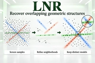 Shared observations, overlapping geometric regions.
Combinatorial explosion in multi-model fitting: Why blind random sampling fails
Multi-model fitting addresses a universal challenge across robotic navigation, 3D scene reconstruction, and spatial computing: real physical environments rarely contain a single clean geometric structure. Instead, dozens of intersecting planar walls, ground surfaces, and boundaries co-exist simultaneously, deeply corrupted by sensor noise and unassociated outliers.
In classical robust estimation, instantiating a candidate geometric hypothesis requires only a minimal sample set of cardinality $m$—for example, $m=2$ points for fitting a 2D line, $m=3$ points for a 3D plane, or $m=8$ correspondences for an epipolar fundamental matrix.
When researchers apply naive random sampling (as in standard RANSAC) to multi-structure scenes, the mathematical foundation of uniform sampling breaks down catastrophically. With dozens of structures co-existing under heavy background outliers, picking two points at random almost invariably draws points from two entirely different physical objects, or samples pure noise. The probability of randomly drawing $m$ points that all belong to the exact same physical structure collapses exponentially as the number of models grows. Yet under classical pipelines, every invalid sample pair is still fed into algebraic solvers and scored across the entire dataset. Computational budgets are overwhelmingly consumed by solving and evaluating hypotheses that were doomed from the start.
Conversely, extending single-model fitters greedily—such as Sequential RANSAC, which fits one model, strips away its inliers, and repeats—introduces hard-assignment clustering distortions. Real structures often share points along intersections and boundaries; greedily stripping inliers deprives adjacent structures of necessary geometric support, causing severe model under-counting and missed detections.
Three further constraints shaped what we built. The method has to work without being told how many models are present, which rules out a family of approaches that take that count as input. It has to run at a usable speed. And it has to transfer across tasks, because a multi-model fitter that has to be re-engineered per problem is not a general tool.
The four things that actually go wrong
We organize the problem around four failure modes, and each component of the method answers one of them.
The first is insufficient utilization of geometric features. Existing methods either rely on hand-designed criteria that only look at part of the geometry, or they are neural networks that never see it explicitly.
The second is inefficient optimization caused by noise. Solver calls are spent on hypotheses that were hopeless from the start.
The third is model overlap, which is the fundamental difference between fitting one model and fitting several, and which most formulations cannot even represent.
The fourth is the non-differentiable pipeline. Discrete minimal-set sampling and the task-specific minimal solver both sit in the middle of the process, and neither has a gradient. Challenges arise in incorporating learning-based methods precisely because of this, and the two available escape routes are both unattractive: replace the exact solver with a differentiable relaxation and lose it, or use policy-gradient estimation and accept the variance.
What competing methods leave unresolved
Greedy single-model extensions carry the hard-assignment problem described above. MultiRANSAC fits K models per iteration instead of one, which requires K as prior knowledge and becomes computationally inefficient as K grows, because finding several good models in a single iteration is genuinely difficult.
Iterative hypothesis generators are the more sophisticated family, and their shared defect is temporal coupling. Because each new model is built on the results of previous iterations, errors accumulate through model overlap as the process proceeds. Our own ablation is honest about the tradeoff here: substituting a stronger learned sampler into LNR raises accuracy and makes the whole process considerably slower. We chose the cheaper option deliberately and we report what it costs.
Clustering-style methods, including preference-set clustering and networks that classify minimal sets as valid or invalid, work well on the problems they target and ignore the reuse of data. Information gathered while evaluating one hypothesis is not carried into the evaluation of another.
Another family replaces sampling heuristics with a global energy function over geometric errors and cluster regularity, or a convex relaxation of the assignment energy, or hypergraph mode-seeking. These formulations handle overlap by construction, and they rely on cost functions complex enough that they may not fully exploit the geometric information actually present in the data. That limits how well they carry across diverse and complex scenes.
Efficient sampling methods that exploit parallel computation are strong, and they need the number of instances as prior information, which limits where they can be applied.
Finally, end-to-end deep methods achieve good accuracy and operate as black boxes. That is a real obstacle to reliable deployment, and it is the specific thing we did not want to build.
Learn at the decisions, condition on the points
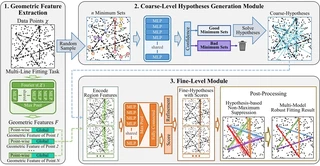
Our approach is to keep the classical pipeline exactly as it is and put learning only where a decision is being made: before solving, to decide which minimal sets deserve a solver call, and after solving, to decide how each hypothesis should move and how good it is.
The critical design choice is what the network is conditioned on. The learned quantities are functions of the geometric features of data points, not of the hypothesis parameters. That is what allows the sampler and the solver to stay in the pipeline as non-differentiable black boxes in the forward pass. No gradient has to pass through either of them.
A precise statement is worth making, because it is easy to overstate. The solver is used during training: the labels for both classifiers come from comparing a solved hypothesis against the ground-truth instance, and the coarse labels come from solving the sampled sets. What does not happen is differentiation through the solver or the sampler. They are used forward-only.
Each point is lifted by a Fourier feature mapping to improve spatial frequency encoding, passed through shared multilayer perceptrons implemented as point-wise convolutions, and max-pooled into a global descriptor. Point-wise and global features are concatenated into a 256-dimensional vector, so every point carries both its own local geometry and a summary of the scene. The coarse module needs that holistic view. The fine module, as it turns out, does not.
Screening before solving
The coarse module draws a large number of minimal sets at random, deliberately more than needed to ensure broad coverage, and predicts a confidence for each. Only the top-scoring sets reach the solver.
Two things about this are worth dwelling on. The first is why the sampling stays random rather than becoming iterative. Random sampling avoids the error accumulation that iterative generators suffer from, and it preserves coverage across the whole observation set. It is a pragmatic choice rather than an optimal one, and we say so.
The second is that the confidence is trained as a binary classification problem, which means the module learns to select promising minimal sets without any explicit degeneracy test. Classical pipelines hand-code checks to reject degenerate configurations. Here that rejection is learned from solved hypotheses compared against ground truth. We replaced a hand-written rule with a learned one, and the benefit is that it adapts to the data rather than to the person who wrote it.
Removing the coarse module hurts significantly, because the fine network cannot cope with the resulting candidate volume. Pretraining the coarse module separately instead of training the two jointly also does worse, and the reason is the most interesting thing in the training design.
Judging a hypothesis by its neighbourhood
For each surviving hypothesis we define a neighbour region: the data points within some range under a task-specific distance. Euclidean distance for lines, a directional distance for vanishing points, reprojection error for planes, the normalized epipolar constraint for motion. The points in that region are encoded, each point’s residual to the hypothesis is concatenated to its features, short regions are zero-padded so they can be batched, and two heads read the result.
One head predicts an increment rather than a model. For a line it predicts a small change to each endpoint. For a vanishing point, a homography or a fundamental matrix it predicts a corresponding adjustment, and that adjustment is added to the coarse hypothesis. The network never invents a model from scratch. Verifying and correcting a guess is easier than generating one, so the classical solver generates and the network corrects.
The other head predicts a score. This is where the paper takes a position that surprises people: consensus maximization does not favour the best model. Counting inliers is the standard proxy for hypothesis quality, and when models overlap it is the wrong proxy. Learning the score from the data around the hypothesis is what replaces it.
The region representation is also what makes overlap representable at all. Two crossing lines have a shared neighbourhood near their intersection, and the points there sit inside both regions and count as evidence for both hypotheses. No hard assignment is made anywhere.
And the fine module deliberately discards the global context that the coarse module relies on. Local details are more relevant for refining an individual hypothesis, and global information can introduce many irrelevant details that hinder the process. The same feature that helps screening hurts refinement. That asymmetry is a reusable coarse-to-fine principle, and it is the reason the two modules are not simply the same network applied twice.
Deciding how many models there are
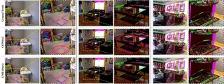
The scored hypotheses are redundant. Several of them will describe the same structure, and the answer should mention it once. We adapted non-maximum suppression from object detection to this setting, replacing intersection-over-union with a geometric notion of similarity: endpoint distance and angle for lines, proximity on the Gaussian sphere for vanishing points, and similarity between the per-point distance vectors for homographies and fundamental matrices.
This is also the mechanism that decides how many models the scene contains. The count is an output of suppression rather than an input to the method, which is what we wanted from the start.
How the two modules train each other
Three losses. The coarse confidence and the fine score are both binary cross-entropy against labels derived from similarity to the ground-truth instance. The refinement head is trained with a smooth L1 objective on the parameter increments.
The coupling is the part worth explaining. The fine-level loss back-propagates into the coarse-level module, so the selector learns to prioritize hypotheses that the fine module is able to work with, rather than simply matching a predefined label. The two modules share the encoded region features, which is what makes the gradient path exist. Training jointly beats pretraining the coarse module, and the reason is that the fine signal reshapes what good means at the coarse stage.
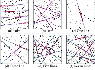
One further observation from the ablations that we did not expect. Training only on harder scenes, with more lines present, matched or beat training on easier ones, and we attribute this to the greater data variability acting as a regularizer. The same effect appeared more weakly for the baseline sampler we compared against.
What we take from this
Decouple learning from non-differentiable components by changing what you condition on rather than by making them differentiable. That refusal is the strongest methodological statement in this work, and it is what preserves the exact solver.
Optimize a selector for downstream compatibility rather than for its own proxy label. Pre-training loses information that joint training keeps.
Consensus is not quality. When models overlap, inlier counting is the wrong measure, and assuming it is right is what causes models to be under-counted.
The value of a feature depends on the stage. Global context helps screening and hurts refinement.
And model the multiplicity structurally. If the interface forces each point into one model, no amount of training will represent two.
What it assumes
The classifiers need supervision in the form of ground-truth instances. Behaviour in a domain with no ground-truth models is not something we characterize.
The region radius and the sampling budget are task-dependent quantities that we do not specify how to set beyond that they vary, and the suppression thresholds are not stated either.
Transfer across tasks means re-deriving four task-specific pieces: the region distance metric, the solver, the refinement parameterization, and the suppression similarity. That is real per-task engineering, and we do not claim zero-shot adaptation.
Zero-padding is our only mechanism for variable-size neighbourhoods, and whether it dilutes the encoding for regions with few points is not something we examined.
And random sampling is a tradeoff rather than an optimum. Our own ablation shows a better sampler would improve accuracy, and we did not resolve whether a cheap learned sampler could get both.
Why keep the two-step pipeline
We kept the established two-step strategy for a specific reason: interpretability. Numerical methods have inherent interpretability and clearly defined application scopes, and they struggle to fully exploit the geometric features of the data. End-to-end deep methods perform well and cannot tell you how they got there.
Because LNR keeps the pipeline, its outputs are explicit geometric models. The network accepts generic unordered data points, covering image correspondences, 3D point clouds and pixel coordinates, and the loss operates on geometric features rather than on hypotheses. That is what maintains compatibility with a broad spectrum of solvers and sampling processes, differentiable or not.
The stated ambition is modest by design. We hope this introduces a new idea for approaching multi-model fitting in a learned way, and we would rather have a method whose behaviour can be interrogated than one whose accuracy we cannot explain.